Comparing Two means (ANOVA and T.test)
Motivation
As a statistics tutor ,One of the question i always encounter is How do i apply statistics in real life , like Zvinoshanda here zvinhu izvi , well the answer is yes. With the rise in popularity of big data , statistical literacy is as important as other literacies . Knowing how to handle and draw conclusions is a must
T-test
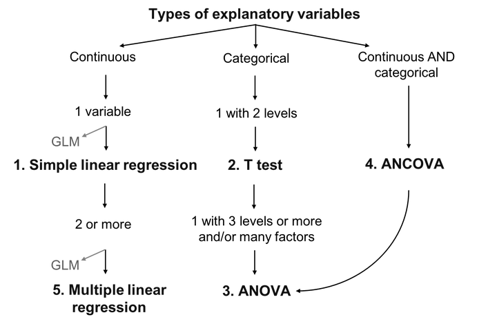
When you have a single explanatory variable which is qualitative and only have two levels, you can run a student’s T-test to test for a difference in the mean of the two levels. If appropriate for your data, you can choose to test a unilateral hypothesis. This means that you can test the more specific assumption that one level has a higher mean than the other, rather than that they simply have different means.Note that robustness of this test increases with sample size and is higher when groups have equal sizes
For the t-test, the t statistic used to find the p-value calculation is calculated as:
\(t = (\overline{y_{1}}-\overline{y_{2}})/\sqrt{\frac{s_{1}^2} n_{1} + \frac{s_{2}^2} n_{2}}\)
where
\(\overline{y_{1}}\) and \(\overline{y_{2}}\) are the means of the response variable y for group 1 and 2, respectively,
\(s_{1}^2\) and \(s_{2}^2\) are the variances of the response variable y for group 1 and 2, respectively,
\(n_{1}\) and \(n_{2}\) are the sample sizes of groups 1 and 2, respectively.
Note that the t-test is mathematically equivalent to a one-way ANOVA with 2 levels.
Assumptions
If the assumptions of the t-test are not met, the test can give misleading results. Here are some important things to note when testing the assumptions of a t-test.
-
Normality of data
As with simple linear regression, the residuals need to be normally distributed. If the data are not normally distributed, but have reasonably symmetrical distributions, a mean which is close to the centre of the distribution, and only one mode (highest point in the frequency histogram) then a t-test will still work as long as the sample is sufficiently large (rule of thumb ~30 observations). If the data is heavily skewed, then we may need a very large sample before a t-test works. In such cases, an alternate non-parametric test should be used. -
Homoscedasticity
Another important assumption of the two-sample t-test is that the variance of your two samples are equal. This allows you to calculate a pooled variance, which in turn is used to calculate the standard error. If population variances are unequal, then the probability of a Type I error is greater than\(\alpha\).
The robustness of the t-test increases with sample size and is higher when groups have equal sizes.
We can test for difference in variances among two populations and ask what is the probability of taking two samples from two populations having identical variances and have the two sample variances be as different as are\(s_{1}^2\)and\(s_{2}^2\).
To do so, we must do the variance ratio test (i.e. an F-test).
Running a t-test (Question from Zou Module)
A psychologist gave a test to 10 females and 10 males to test the hypothesis that males should score higher on the tests. The following scores were obtained.
Females<- c(20,	15,	19,	18,13,	14,	16,	12,	15,	25)
Males<-c(20	,16	,24	,11	,23,	25,	22,	24,	26,	28)

df<-cbind(Females,Males) %>%
   data.frame()

df %>% rownames_to_column(var = " ") %>%
  janitor::adorn_totals(where = c("row", "col")) %>%
  flextable::flextable() %>%
  flextable::colformat_int(j = c(2, 3, 4), big.mark = ",") %>%
  flextable::autofit()
| Females | Males | Total |
|---|---|---|---|
1 | 20 | 20 | 40 |
2 | 15 | 16 | 31 |
3 | 19 | 24 | 43 |
4 | 18 | 11 | 29 |
5 | 13 | 23 | 36 |
6 | 14 | 25 | 39 |
7 | 16 | 22 | 38 |
8 | 12 | 24 | 36 |
9 | 15 | 26 | 41 |
10 | 25 | 28 | 53 |
Total | 167 | 219 | 386 |
Assuming that the populations are normal with equal variance test the claim at 5% level of Significance run a t test. (20).
In R
- R understands both the t.test and anova more oftenly in long format rather than wide format
df_new<-df |>
  gather("gender","value")
ggplot(df_new,aes(x=gender,y=value,fill=gender))+geom_boxplot()

There seem to be a difference just by looking at the boxplot. Let’s make sure are assumptions are met before doing the test.
# Assumption of equal variance
vattest<-var.test(value~gender,data=df_new)
vattest
#>
#> 	F test to compare two variances
#>
#> data:  value by gender
#> F = 0.58943, num df = 9, denom df = 9, p-value = 0.4431
#> alternative hypothesis: true ratio of variances is not equal to 1
#> 95 percent confidence interval:
#>  0.1464067 2.3730524
#> sample estimates:
#> ratio of variances
#>          0.5894327
comment
vattest$p.value
#> [1] 0.4431275
the p-value is greater than 0.05 indicating theat that there is no significance difference in the variances for males and females.
vattest$estimate
#> ratio of variances
#>          0.5894327
the ratio is also close to one hence the assumption of homogeniety holds
Running the test mannually
$$\bar{X}_{males}=21.9$$ $$\bar{X}_{females}=16.7$$
Hypothesis
- H0:
\(\bar{X}_{males}=\bar{X}_{females}\) - H1:
\(\bar{X}_{males}>\bar{X}_{females}\)
$$S^2_{females}=\frac{\sum(x-\bar{x}_{females})^2}{n-1}$$
$$S^2_{females}=\frac{(20-16.7)^2+(15-16.7)^2+...+(25-16.7)^2}{9}=15.12222$$
$$S^2_{males}=\frac{\sum(x-\bar{x}_{males})^2}{n-1}$$
$$S^2_{males}=\frac{(20-21.9)^2+(16-21.9)^2+...+(28-21.9)^2}{9}=25.65556$$
$$S_{pooled}=\frac{(N_{males}-1)S^2_{males}+(N_{females}-1)S^2_{females}}{N_{males}+N_{females}-2}$$
$$S_{pooled}=\frac{(9)(25.65556)+(9)(15.12222)}{18}=20.38889$$
test statistic
$$t=\frac{\bar{X}_{males}-\bar{X}_{females}}{S_{pooled}(\frac{1}{N_{males}}+\frac{1}{N_{females}})}$$
$$t=\frac{21.9-16.7}{20.38889(2/10)}=2.575085$$
$$t_{0.05}(18)=1.734$$
Conclusion
since \(t>t_{0.05}(18)\) we reject the null hypothesis and conclude that
there is evidence to prove that the means are not equal and suggest that
the average for males is greater than that of females.
In R, t-tests are implemented using the function t.test.
t.test(Y ~ X2, data= data, alternative = c("greater","less","two.sided"),var.equal=TRUE)
# or equivalently
ttest1 <- t.test(value~gender, var.equal=TRUE,alternative="greater",data=df_new)
ttest1
#>
#> 	Two Sample t-test
#>
#> data:  value by gender
#> t = -2.5751, df = 18, p-value = 0.9905
#> alternative hypothesis: true difference in means between group Females and group Males is greater than 0
#> 95 percent confidence interval:
#>  -8.701683       Inf
#> sample estimates:
#> mean in group Females   mean in group Males
#>                  16.7                  21.9
var.equal=TRUE implies we are enforcing the restriction that the variances are equal
-1*ttest1$statistic
#>        t
#> 2.575085
this is the value we calculated earlier
ttest1$p.value
#> [1] 0.9904643
the p-value is greater than 0.05 hence we conclude that the true difference in means between group Females and group Males is greater than 0
Analysis of Variance (ANOVA)
Analysis of Variance (ANOVA) is a type of linear model for a continuous
response variable and one or more categorical explanatory variables. The
categorical explanatory variables can have any number of levels
(groups). For example, the variable race might have three levels:
Black,White and Hispanic. ANOVA tests whether the means of the response
variable differ between the levels by comparing the variation within a
group with the variation among groups. For example, if mean IQ for those who are black differs with those who are white.
ANOVA calculations are based on the sum of squares partitioning and
compares the :
-
within-level varianceto the -
between-level variance.
If the between-level variance is greater than the within-level variance, this means that the levels affect the explanatory variable more than the random error (corresponding to the within-level variance), and that the explanatory variable is likely to be significantly influenced by the levels.

Doing the calculation
In the ANOVA, the comparison of the between-level variance to the
within-level variance is made through the calculation of the
F-statistic that correspond to the ratio of the mean sum of squares of
the level (MSLev) on the mean sum of squares of the error (MS$\epsilon$).
These two last terms are obtained by dividing their two respective sums
of squares by their corresponding degrees of freedom, as is typically
presented in a ANOVA table . Finally, the p-value of the ANOVA is calculated
from the F-statistic that follows a Chi-square (χ2) distribution.
Anova Table
| Source of variation |
Degrees of freedom (df) |
Sums of squares | Mean squares | F-statistic | |
|---|---|---|---|---|---|
| Total | \(ra-1\) |
\(SS_{t}=\sum x^2 - \frac{G^2}{N}\) |
|||
| Facteur A | \(a-1\) |
\(SS_{f}=\frac{\sum{T_j^2}}{n}-\frac{G^2}{N}\) |
\(MS_{f}=\frac{SS_{f}}{(a-1)}\) |
`(F= {MS_{ | E}})` |
| Error | \(a(r-1)\) |
\(SS_{\epsilon}=SS_{total} – SS_{group}\) |
`(MS_{}=\frac{SS_{}}{a( | r-1)})` |
let \(T_j\) be total for the \(j_{th}\) group and
Grand total=G
QUESTION
To investigate maternal behavior of laboratory rats, we separated the rat pup from the mother and recorded the time (in seconds) required for the mother to retrieve the pup. We ran the study with 5-, 20-, and 35 – day – old pups because we were interested in whether retrieval time various with the age of pup. The data are given below, where there are six pups per group.
| day 5 | day 20 | day 35 |
|---|---|---|
| 10 | 15 | 35 |
| 15 | 30 | 40 |
| 25 | 20 | 50 |
| 15 | 15 | 43 |
| 20 | 23 | 45 |
| 18 | 20 | 40 |
| 103 | 123 | 253 |
Calculating the test statistic
let \(T_j\) be total for the \(j_{th}\) group \(T_5=103\) ,$T_{20}=123$ and
\(T_{35}=253\) Grand total=G=103+123+253=479
$$SS_{total}=\sum x^2 - \frac{G^2}{N}$$
$$SS_{total} =(10^2+15^2+25^2+ ... + 45^2+40^2)-479^2/18=15377-12746.72$$
$$SS_{total}=2630.278$$
$$SS_{group}=\frac{\sum{T_j^2}}{n}-\frac{G^2}{N}$$
$$SS_{group}=\frac{103^2+123^2+253^2}{6}-\frac{479^2}{18}$$
$$SS_{group}=\frac{89747}{6}-\frac{479^2}{18}$$ $$SS_{group}=2211.111$$
$$SS_{error} = SS_{total} – SS_{group}$$
$$SS_{error} = 419.167$$
| Source | df | SS | MS | F |
|---|---|---|---|---|
| Groups | 2 | 2211.111 | 1105.555 | 39.56257 |
| Error | 15 | 419.167 | 27.94447 | |
| Total | 17 | 2630.278 | 154.7222 |
Define the hypothesis
- H0 : all Means are equal
- H1 : At least one mean is different
critical value
$$F_{2,15}(0.05)=3.68$$
Conclusion
Because our obtained F = 39.56257 exceeds
\(F_{.05} = 3.68\), we will reject \(H_0\) and conclude that the groups were
sampled from populations with different means.
Doing this in R
library(tidyverse)
df<-tribble(~DAY_5 ,~DAY_20,~DAY_35,
 	10,	15,	35,
 	15,	30,	40,
 	25,	20,	50,
 	15,	15,	43,
 	20,	23,	45,
 	18,	20,	40)
df
#> # A tibble: 6 x 3
#>   DAY_5 DAY_20 DAY_35
#>   <dbl>  <dbl>  <dbl>
#> 1    10     15     35
#> 2    15     30     40
#> 3    25     20     50
#> 4    15     15     43
#> 5    20     23     45
#> 6    18     20     40
Look at the means
sapply(df,mean)
#>    DAY_5   DAY_20   DAY_35
#> 17.16667 20.50000 42.16667
look at the standard deviation
sapply(df,sd)
#>    DAY_5   DAY_20   DAY_35
#> 5.115336 5.612486 5.115336
Change to long format
out_new<-df |>
  gather("day","time")
visually inspect
ggplot(out_new,aes(x=day,y=time,fill=day))+geom_boxplot()

Let’s now run the ANOVA. In R, ANOVA can be called either directly with the aov function, or with the anova function performed on a linear model implemented with lm:
# Using aov()
aov1 <- aov(time ~ day, data=out_new)
summary(aov1)
#>             Df Sum Sq Mean Sq F value   Pr(>F)
#> day          2 2211.1  1105.6   39.56 1.04e-06 ***
#> Residuals   15  419.2    27.9
#> ---
#> Signif. codes:  0 '***' 0.001 '**' 0.01 '*' 0.05 '.' 0.1 ' ' 1

# Using lm()
anov1 <- lm(time ~ day, data=out_new)
anova(anov1)
#> Analysis of Variance Table
#>
#> Response: time
#>           Df  Sum Sq Mean Sq F value    Pr(>F)
#> day        2 2211.11 1105.56  39.563 1.042e-06 ***
#> Residuals 15  419.17   27.94
#> ---
#> Signif. codes:  0 '***' 0.001 '**' 0.01 '*' 0.05 '.' 0.1 ' ' 1
breaking down the output (Conclusion from R)
- F-value=39.56 just as we calculated before
- Pr(F) is less than 5 percent indicating that the means are significantly different
Complementary test
Importantly, ANOVA cannot identify which treatment is different from the
others in terms of response variable. It can only identify that a
difference is present. To determine the location of the difference(s),
post-hoc tests that compare the levels of the explanatory variables
(i.e. the treatments) two by two, must be performed. While several
post-hoc tests exist (e.g. Fischer’s least significant difference,
Duncan’s new multiple range test, Newman-Keuls method, Dunnett’s test,
etc.), the Tukey’s range test is used in this example using the function
TukeyHSD as follows:
# Where does the Diet difference lie?
TukeyHSD(aov(anov1),ordered=T)

# or equivalently
TukeyHSD(aov1,ordered=T)
Conclusion
- looking at the column with p adj , values that are less than
0.05indicate that the pair has a significant difference in means thus pairsDAY_35-DAY_5andDAY_35-DAY_20are are significant
the plot
tkplot<-TukeyHSD(aov1,ordered=T)
plot(tkplot)

Bongani Ncube
Data Scientist/Statistics/Public Health
My research interests include Casual Inference , Public Health , Survival Analysis, bayesian Statistics, Machine learning and Longitudinal Data Analysis.