Base R vs dplyr vs data.table

Last updated on Sep 17, 2023 13 min read dplyr, wrangling, munging, querying

Introduction

One of the many reasons why people do not like R is because you find more than one way of performing an operation. But i woul like to say this could be an advantage as every possible way can have more advantage for a given task . for instance:

one could find base R syntax very boring
one sees dplyr syntax more intuitive
data.table on the other hand is very fast in terms of performing operations

this blog compares the syntax for base r ,tidyverse and data.table for performing certain operations

library setup

library(data.table)
library(tidyverse)
library(sqldf)

Reading in data

Base R

base R uses the read.csv() function

df_base<-read.csv("loan_data_cleaned.csv")
df_base |> head(n=12)
#>     X loan_status loan_amnt grade home_ownership annual_inc age emp_cat  ir_cat
#> 1   1           0      5000     B           RENT      24000  33    0-15    8-11
#> 2   2           0      2400     C           RENT      12252  31   15-30 Missing
#> 3   3           0     10000     C           RENT      49200  24    0-15 11-13.5
#> 4   4           0      5000     A           RENT      36000  39    0-15 Missing
#> 5   5           0      3000     E           RENT      48000  24    0-15 Missing
#> 6   6           0     12000     B            OWN      75000  28    0-15 11-13.5
#> 7   7           1      9000     C           RENT      30000  22    0-15 11-13.5
#> 8   8           0      3000     B           RENT      15000  22    0-15    8-11
#> 9   9           1     10000     B           RENT     100000  28    0-15    8-11
#> 10 10           0      1000     D           RENT      28000  22    0-15   13.5+
#> 11 11           0     10000     C           RENT      42000  23    0-15 Missing
#> 12 12           0      3600     A       MORTGAGE     110000  27    0-15     0-8

df_base |> 
  summarise_if(is.character,n_distinct) |> 
  t()
#>                [,1]
#> grade             7
#> home_ownership    4
#> emp_cat           5
#> ir_cat            5

tidyverse

readr package from the tidyverse contains the function read_csv()

df_tidy<-read_csv("loan_data_cleaned.csv")
df_tidy |> head(n=12)
#> # A tibble: 12 x 9
#>     ...1 loan_status loan_amnt grade home_ownership annual_inc   age emp_cat
#>    <dbl>       <dbl>     <dbl> <chr> <chr>               <dbl> <dbl> <chr>  
#>  1     1           0      5000 B     RENT                24000    33 0-15   
#>  2     2           0      2400 C     RENT                12252    31 15-30  
#>  3     3           0     10000 C     RENT                49200    24 0-15   
#>  4     4           0      5000 A     RENT                36000    39 0-15   
#>  5     5           0      3000 E     RENT                48000    24 0-15   
#>  6     6           0     12000 B     OWN                 75000    28 0-15   
#>  7     7           1      9000 C     RENT                30000    22 0-15   
#>  8     8           0      3000 B     RENT                15000    22 0-15   
#>  9     9           1     10000 B     RENT               100000    28 0-15   
#> 10    10           0      1000 D     RENT                28000    22 0-15   
#> 11    11           0     10000 C     RENT                42000    23 0-15   
#> 12    12           0      3600 A     MORTGAGE           110000    27 0-15   
#> # i 1 more variable: ir_cat <chr>

using data.table

data.table has the function fread() for handling csv file.

df_table<-fread("loan_data_cleaned.csv")
df_table |> head(n=12)
#>     V1 loan_status loan_amnt grade home_ownership annual_inc age emp_cat
#>  1:  1           0      5000     B           RENT      24000  33    0-15
#>  2:  2           0      2400     C           RENT      12252  31   15-30
#>  3:  3           0     10000     C           RENT      49200  24    0-15
#>  4:  4           0      5000     A           RENT      36000  39    0-15
#>  5:  5           0      3000     E           RENT      48000  24    0-15
#>  6:  6           0     12000     B            OWN      75000  28    0-15
#>  7:  7           1      9000     C           RENT      30000  22    0-15
#>  8:  8           0      3000     B           RENT      15000  22    0-15
#>  9:  9           1     10000     B           RENT     100000  28    0-15
#> 10: 10           0      1000     D           RENT      28000  22    0-15
#> 11: 11           0     10000     C           RENT      42000  23    0-15
#> 12: 12           0      3600     A       MORTGAGE     110000  27    0-15
#>      ir_cat
#>  1:    8-11
#>  2: Missing
#>  3: 11-13.5
#>  4: Missing
#>  5: Missing
#>  6: 11-13.5
#>  7: 11-13.5
#>  8:    8-11
#>  9:    8-11
#> 10:   13.5+
#> 11: Missing
#> 12:     0-8

data wrangling and processing

for reproducibilty we will sample only 30 rows for working with

set.seed(23456)
df_tidy <- df_tidy |> sample_n(size=30)
df_base <- df_tidy |> as.data.frame()
df_table<- df_tidy |> as.data.table()

selecting columns

Base R

base R use df[row,column] syntax to filter rows or columns
we can use indices or column names to do this

## selecting the columns
df_base[,c("loan_amnt","loan_status","grade")]
#>    loan_amnt loan_status grade
#> 1       2650           0     C
#> 2      13000           1     B
#> 3      16750           0     C
#> 4       2500           0     C
#> 5      12000           0     C
#> 6       5000           0     B
#> 7       7000           0     C
#> 8      12000           0     C
#> 9      12000           0     A
#> 10      7000           0     A
#> 11      7500           0     C
#> 12     19000           0     B
#> 13     15000           0     B
#> 14      9600           0     A
#> 15     20000           0     A
#> 16     10000           0     A
#> 17     10000           0     B
#> 18      7000           0     E
#> 19     15000           0     A
#> 20     11000           0     A
#> 21      6000           0     C
#> 22      6000           0     B
#> 23      5400           0     A
#> 24     10000           1     D
#> 25      9900           0     B
#> 26      9000           0     B
#> 27     17500           0     D
#> 28      2550           0     B
#> 29      9000           0     A
#> 30      1000           0     C

tidyverse

dplyr package contains the select statement that is used to call of the required variables

## use select statement
df_tidy |> select(loan_amnt,loan_status,grade)
#> # A tibble: 30 x 3
#>    loan_amnt loan_status grade
#>        <dbl>       <dbl> <chr>
#>  1      2650           0 C    
#>  2     13000           1 B    
#>  3     16750           0 C    
#>  4      2500           0 C    
#>  5     12000           0 C    
#>  6      5000           0 B    
#>  7      7000           0 C    
#>  8     12000           0 C    
#>  9     12000           0 A    
#> 10      7000           0 A    
#> # i 20 more rows

data.table

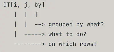
data.table uses Almost the same syntax as the data.frame is selecting columns
it uses the syntax DT[i,j,k]
for columns the two are typically the same

## selecting columns
df_table[,c("loan_amnt","loan_status","grade")]
#>     loan_amnt loan_status grade
#>  1:      2650           0     C
#>  2:     13000           1     B
#>  3:     16750           0     C
#>  4:      2500           0     C
#>  5:     12000           0     C
#>  6:      5000           0     B
#>  7:      7000           0     C
#>  8:     12000           0     C
#>  9:     12000           0     A
#> 10:      7000           0     A
#> 11:      7500           0     C
#> 12:     19000           0     B
#> 13:     15000           0     B
#> 14:      9600           0     A
#> 15:     20000           0     A
#> 16:     10000           0     A
#> 17:     10000           0     B
#> 18:      7000           0     E
#> 19:     15000           0     A
#> 20:     11000           0     A
#> 21:      6000           0     C
#> 22:      6000           0     B
#> 23:      5400           0     A
#> 24:     10000           1     D
#> 25:      9900           0     B
#> 26:      9000           0     B
#> 27:     17500           0     D
#> 28:      2550           0     B
#> 29:      9000           0     A
#> 30:      1000           0     C
#>     loan_amnt loan_status grade

however data.table() often uses the syntax .() for filtering and selecting

df_table[,.(loan_amnt,loan_status,grade)]
#>     loan_amnt loan_status grade
#>  1:      2650           0     C
#>  2:     13000           1     B
#>  3:     16750           0     C
#>  4:      2500           0     C
#>  5:     12000           0     C
#>  6:      5000           0     B
#>  7:      7000           0     C
#>  8:     12000           0     C
#>  9:     12000           0     A
#> 10:      7000           0     A
#> 11:      7500           0     C
#> 12:     19000           0     B
#> 13:     15000           0     B
#> 14:      9600           0     A
#> 15:     20000           0     A
#> 16:     10000           0     A
#> 17:     10000           0     B
#> 18:      7000           0     E
#> 19:     15000           0     A
#> 20:     11000           0     A
#> 21:      6000           0     C
#> 22:      6000           0     B
#> 23:      5400           0     A
#> 24:     10000           1     D
#> 25:      9900           0     B
#> 26:      9000           0     B
#> 27:     17500           0     D
#> 28:      2550           0     B
#> 29:      9000           0     A
#> 30:      1000           0     C
#>     loan_amnt loan_status grade

filtering rows

Base R

typically you need to specify row range for this operation
DF[range,]
code below will only take rows 1,2,3,5 and 10

df_base[c(1:3,5,10),]
#>     ...1 loan_status loan_amnt grade home_ownership annual_inc age emp_cat
#> 1  17445           0      2650     C       MORTGAGE      86000  28    0-15
#> 2  12396           1     13000     B       MORTGAGE      31000  32    0-15
#> 3  26032           0     16750     C       MORTGAGE      45000  23    0-15
#> 5   3564           0     12000     C       MORTGAGE     160000  40    0-15
#> 10 19236           0      7000     A           RENT      18000  23    0-15
#>     ir_cat
#> 1  11-13.5
#> 2  Missing
#> 3  11-13.5
#> 5    13.5+
#> 10     0-8

Tidyverse

dplyr uses the slice or filter function to achieve the same as above

df_tidy |> slice(1:3,5,10)
#> # A tibble: 5 x 9
#>    ...1 loan_status loan_amnt grade home_ownership annual_inc   age emp_cat
#>   <dbl>       <dbl>     <dbl> <chr> <chr>               <dbl> <dbl> <chr>  
#> 1 17445           0      2650 C     MORTGAGE            86000    28 0-15   
#> 2 12396           1     13000 B     MORTGAGE            31000    32 0-15   
#> 3 26032           0     16750 C     MORTGAGE            45000    23 0-15   
#> 4  3564           0     12000 C     MORTGAGE           160000    40 0-15   
#> 5 19236           0      7000 A     RENT                18000    23 0-15   
#> # i 1 more variable: ir_cat <chr>

data.table way

df_table[c(1:3,5,10),]
#>     ...1 loan_status loan_amnt grade home_ownership annual_inc age emp_cat
#> 1: 17445           0      2650     C       MORTGAGE      86000  28    0-15
#> 2: 12396           1     13000     B       MORTGAGE      31000  32    0-15
#> 3: 26032           0     16750     C       MORTGAGE      45000  23    0-15
#> 4:  3564           0     12000     C       MORTGAGE     160000  40    0-15
#> 5: 19236           0      7000     A           RENT      18000  23    0-15
#>     ir_cat
#> 1: 11-13.5
#> 2: Missing
#> 3: 11-13.5
#> 4:   13.5+
#> 5:     0-8

filtering both rows and columns

Base R

df_base[c(1:3,5,10),c("loan_amnt","loan_status","grade")]
#>    loan_amnt loan_status grade
#> 1       2650           0     C
#> 2      13000           1     B
#> 3      16750           0     C
#> 5      12000           0     C
#> 10      7000           0     A

perhaps you want to filter rows where grade is A and loan_status is 0 for the columns grade,loan_status and loan_amnt

df_base[df_base$grade=="A"& df_base$loan_status==0,c("loan_amnt","loan_status","grade")]
#>    loan_amnt loan_status grade
#> 9      12000           0     A
#> 10      7000           0     A
#> 14      9600           0     A
#> 15     20000           0     A
#> 16     10000           0     A
#> 19     15000           0     A
#> 20     11000           0     A
#> 23      5400           0     A
#> 29      9000           0     A

tidyverse way

dplyr contains the filter function useful for filtering data
it can be used with the slice function to obtain results below

df_tidy |> 
  slice(1:3,5,10) |> 
  select(loan_amnt,loan_status,grade)
#> # A tibble: 5 x 3
#>   loan_amnt loan_status grade
#>       <dbl>       <dbl> <chr>
#> 1      2650           0 C    
#> 2     13000           1 B    
#> 3     16750           0 C    
#> 4     12000           0 C    
#> 5      7000           0 A

perhaps you wish to filter based on some particular condition

df_tidy |> 
  select(loan_status,loan_amnt,grade) |> 
  filter(grade=="A"& loan_status==0)
#> # A tibble: 9 x 3
#>   loan_status loan_amnt grade
#>         <dbl>     <dbl> <chr>
#> 1           0     12000 A    
#> 2           0      7000 A    
#> 3           0      9600 A    
#> 4           0     20000 A    
#> 5           0     10000 A    
#> 6           0     15000 A    
#> 7           0     11000 A    
#> 8           0      5400 A    
#> 9           0      9000 A

data.table way

unlike in the data.frame , we dont have to index using a $ operator

df_table[grade=="A"& loan_status==0,.(loan_amnt,loan_status,grade)]
#>    loan_amnt loan_status grade
#> 1:     12000           0     A
#> 2:      7000           0     A
#> 3:      9600           0     A
#> 4:     20000           0     A
#> 5:     10000           0     A
#> 6:     15000           0     A
#> 7:     11000           0     A
#> 8:      5400           0     A
#> 9:      9000           0     A

data exploration

helper filters

expressions for finding matches
lets use a different dataset for this

set.seed(9898)
df<-read_csv("recipe_site_traffic_2212.csv") |> 
  sample_n(size=50)
tidyv<-df
baseR<-df |> as.data.frame()
datatab<-df |> as.data.table()

base R

grepl function is useful for dealing with character expressions
the following expression will filter the rows that category matching the expression hicken

baseR[grepl("hicken",baseR$category),c("recipe","category","calories")]
#>    recipe       category calories
#> 4     180 Chicken Breast   410.34
#> 13    906 Chicken Breast    42.30
#> 24    892        Chicken   309.67
#> 28    741 Chicken Breast  1402.99
#> 29    053        Chicken   367.30
#> 30    570        Chicken   531.11
#> 33    169 Chicken Breast  1044.92
#> 39    657 Chicken Breast   458.66
#> 40    502        Chicken   883.12
#> 43    682 Chicken Breast   339.38
#> 46    529 Chicken Breast   196.69

tidyverse

we can use str_detect or str_like from stringr and filter function

tidyv |> 
  filter(str_like(category,"Chicken%")) |> 
  select(recipe,category,calories)
#> # A tibble: 11 x 3
#>    recipe category       calories
#>    <chr>  <chr>             <dbl>
#>  1 180    Chicken Breast    410. 
#>  2 906    Chicken Breast     42.3
#>  3 892    Chicken           310. 
#>  4 741    Chicken Breast   1403. 
#>  5 053    Chicken           367. 
#>  6 570    Chicken           531. 
#>  7 169    Chicken Breast   1045. 
#>  8 657    Chicken Breast    459. 
#>  9 502    Chicken           883. 
#> 10 682    Chicken Breast    339. 
#> 11 529    Chicken Breast    197.

data.table

we can use the %like% function to detect matches in expressions

datatab[category %like% "^Chicken",.(recipe,category,calories)]
#>     recipe       category calories
#>  1:    180 Chicken Breast   410.34
#>  2:    906 Chicken Breast    42.30
#>  3:    892        Chicken   309.67
#>  4:    741 Chicken Breast  1402.99
#>  5:    053        Chicken   367.30
#>  6:    570        Chicken   531.11
#>  7:    169 Chicken Breast  1044.92
#>  8:    657 Chicken Breast   458.66
#>  9:    502        Chicken   883.12
#> 10:    682 Chicken Breast   339.38
#> 11:    529 Chicken Breast   196.69

filtering ranges

say you want to take only rows where calories are in the range of 500 to 800

base R

baseR[baseR$calories>=500 & baseR$calories<=800,c("recipe","category","calories")]
#>    recipe      category calories
#> 3     575          Meat   504.20
#> 17    028        Potato   574.75
#> 25    602        Potato   565.23
#> 27    183     Vegetable   699.44
#> 30    570       Chicken   531.11
#> 31    068     Breakfast   717.72
#> 32    437 One Dish Meal   726.23
#> NA   <NA>          <NA>       NA
#> 37    276  Lunch/Snacks   597.55
#> 44    266        Potato   626.61
#> 48    402  Lunch/Snacks   633.87

tidyverse

tidyv |> 
  filter(between(calories,500,800)) |> 
  select(recipe,category,calories)
#> # A tibble: 10 x 3
#>    recipe category      calories
#>    <chr>  <chr>            <dbl>
#>  1 575    Meat              504.
#>  2 028    Potato            575.
#>  3 602    Potato            565.
#>  4 183    Vegetable         699.
#>  5 570    Chicken           531.
#>  6 068    Breakfast         718.
#>  7 437    One Dish Meal     726.
#>  8 276    Lunch/Snacks      598.
#>  9 266    Potato            627.
#> 10 402    Lunch/Snacks      634.

data.table

datatab[calories %between% c(500,800),.(recipe,category,calories)]
#>     recipe      category calories
#>  1:    575          Meat   504.20
#>  2:    028        Potato   574.75
#>  3:    602        Potato   565.23
#>  4:    183     Vegetable   699.44
#>  5:    570       Chicken   531.11
#>  6:    068     Breakfast   717.72
#>  7:    437 One Dish Meal   726.23
#>  8:    276  Lunch/Snacks   597.55
#>  9:    266        Potato   626.61
#> 10:    402  Lunch/Snacks   633.87

summarizing data

Base R

mean(baseR$calories,na.rm = T)
#> [1] 371.9794

Tidyverse

tidyv |> 
  summarise(average=mean(calories,na.rm = T))
#> # A tibble: 1 x 1
#>   average
#>     <dbl>
#> 1    372.

data.table

datatab[,mean(calories,na.rm=T)]
#> [1] 371.9794

summarise on filters

say you want to summarize after filtering the data
the code below will find mean calories for rows that match chicken

base R

mean(baseR[grepl("hicken",baseR$category),"calories"],na.rm = T)
#> [1] 544.2255

tidyverse

tidyv |> 
  filter(str_like(category,"Chicken%")) |> 
  summarise(average=mean(calories,na.rm = T))
#> # A tibble: 1 x 1
#>   average
#>     <dbl>
#> 1    544.

data.table

datatab[category %like% "^Chicken",mean(calories,na.rm=T)]
#> [1] 544.2255

Advanced computations

grouping and summarizing

sometimes you wish to perfom some rigorus calculations in either the three methods

Base R

Base R has a powerful function named aggregate that can be used for grouping summarising

aggregate(calories~category,data=baseR,FUN=mean)
#>          category calories
#> 1       Beverages 130.9933
#> 2       Breakfast 335.3967
#> 3         Chicken 522.8000
#> 4  Chicken Breast 556.4686
#> 5         Dessert 857.3400
#> 6    Lunch/Snacks 484.2667
#> 7            Meat 292.6214
#> 8   One Dish Meal 587.4100
#> 9            Pork 113.9520
#> 10         Potato 382.9420
#> 11      Vegetable 325.9267

tidyverse

tidyv |> 
  group_by(category) |> 
  summarise(mean_cal=mean(calories,na.rm = T))
#> # A tibble: 11 x 2
#>    category       mean_cal
#>    <chr>             <dbl>
#>  1 Beverages          131.
#>  2 Breakfast          335.
#>  3 Chicken            523.
#>  4 Chicken Breast     556.
#>  5 Dessert            857.
#>  6 Lunch/Snacks       484.
#>  7 Meat               293.
#>  8 One Dish Meal      587.
#>  9 Pork               114.
#> 10 Potato             383.
#> 11 Vegetable          326.

data.table

datatab[,.(mean_cal=mean(calories,na.rm=T)),by=.(category)]
#>           category mean_cal
#>  1:   Lunch/Snacks 484.2667
#>  2:      Beverages 130.9933
#>  3:           Meat 292.6214
#>  4: Chicken Breast 556.4686
#>  5:  One Dish Meal 587.4100
#>  6:           Pork 113.9520
#>  7:      Vegetable 325.9267
#>  8:      Breakfast 335.3967
#>  9:         Potato 382.9420
#> 10:        Chicken 522.8000
#> 11:        Dessert 857.3400

Bongani Ncube

Data Scientist/Statistics/Public Health

My research interests include Casual Inference , Public Health , Survival Analysis, bayesian Statistics, Machine learning and Longitudinal Data Analysis.